Large Language Models (LLMs) have already revolutionised the way we process text. It is no longer a question of whether we should use an LLM in an NLP application? but rather which one to use? The selection is vast and new models pop-up everyday, which makes it extremely difficult to keep up with the progress in the field. How is this new model different from (or similar to) the other ones?, how likely it will give a different (possibly better) performance on the task that I am interested in? are the type of questions/decisions that practitioner are faced with in modern-day research and development scenarios. We are practically lost in this vast space of LLMs.
What do we do when we are lost? – We create maps!
Following this spirit, we build a map of sentence encoders to visualise their landscape, reflecting the behavioural relationships among 1,101 encoder models. I will present this work at ACL 2026 main conference (oral session) on 5th of July, In this article, I will provide a slightly less technical and more intuitive narration of the idea.
Lets then get lost in the land of LLM encoders, shall we?
What are sentence encoders?
Representing the meaning of sentences is arguably one of the most fundamental quests in NLP. If you can represent the meaning of a sentence in a way that a computer can understand the sentence, then you have (almost) solved the language understanding problem. Models that take in sentences as the input and return vectors (embeddings) as the output are commonly known as sentence encoders. By extension, we can consider text documents as a collection of sentences, so if we have an accurate and reliable method to represent sentences then we can recursively apply it to create representations for documents as well. Many modern day NLP applications such as information retrieval, document classification (e.g. sentiment classification, spam email filtering), document clustering (e.g. grouping similar documents such as news articles on the same genre) etc. depend on accurate sentence/document representations. Indeed one can argue that all machine learning applications that deal with texts require some form of a representation of the input texts and sentence encoders act as the working horses in these applications.
Why is it difficult to map sentence encoders?
OK. We hope you are convinced by now that sentence encoders play a major role in NLP applications. Although we call all types of text encoders as sentence encoders here, it is noteworthy that it is a highly diverse space with lots of different techniques. All sentence encoders solve one fundamental problem – how to represent a variable length sentence using a fixed dimensional vector?
Sentences do come in all forms – there are short ones as well as very very long ones that can even span an entire paragraph. ML algorithms such as classification algorithms expect all instances to be represented over the same set of features (i.e. the feature space is fixed and finite). Therefore, we cannot have different length embeddings coming out from the same sentence encoder for different sentences. There are various ways to overcome this issue, varying in complexity. For example, one could first represent all words in a vocabulary (e.g. as listed in the Oxford English dictionary) by fixed dimensional word embeddings, and then simply add up the word embeddings for the words in a given sentence to create a sentence embedding. Even this simple approach works surprisingly well in many NLP tasks, especially when the word order does not convey significant meaning alternations (Arora+ 2017). However, this averaging of word embeddings (technically known as mean pooling) misses the point hard when the word order in a sentence convey a very different meanings such as in Jack killed Mary vs. Mary killed Jack, potentially deciding the fate of a poor soul. Modern transformer-based methods use attention scores and positional embeddings to incorporate word order into the sentence embeddings to overcome this issue.
But each sentence encoder is a unique creature that has very different properties that make their comparisons notoriously difficult. Specifically, the challenges involved when mapping sentence encoders boil down to three main reasons as follows:
- Multi-variatedness – By construction, sentence encoders return vectors that have many dimensions. Typical modern sentence encoder dimensionalities can range from 256 to 4096 dimensions or more. For example, when considering LLM decoders (sentence generators), we can use the likelihood scores returned by the decoder for a fixed set ($\mathcal{S}$) of sentences (say $N$ sentences) to obtain an $N$-dimensional likelihood vector for representing a given LLM decoder (Oyama+ 2025). We can then compare two decoder models, for example, by the Euclidean distance computed using their likelihood vectors. But LLM encoders (such as the sentence encoders we have been discussing so far) return a vector per sentence, not a scalar value such as the likelihood.
- Mis-aliged vector spaces – Sentence encoders are trained independently, so the embeddings they return live it totally different vector spaces (even when their dimensionalities are be equal). You cannot compare apples to oranges. We need some way to translate one vector space to another before we can even start to compare them meaningfully.
- Dimensionality Mis-match – Different sentence encoders often return embeddings with different dimensionalities. One encoder might return a 768 dimensional representations for a given sentence, while another would return a 1024 dimensional one. None of the dimensions in the first space exist (in general) in the second one. How can we compare vectors of different dimensionalities?
All three above-mentioned difficulties make any direct comparison of sentence encoders challenging. In particular, we need to develop a method for representing each encoder in a dimensionality-independent and embedding-space independent manner first. We then need to come up with a metric that would enable us to accurately and faithfully compare encoder representations. The next two sections tackle these challenges.
Solving the Representational Challenge
Recall that what basically prevents us from comparing two different independently trained encoders is that their embeddings lie in totally different vector spaces. One straightforward approach to tackle this issue would be to learn a transformation from one vector space to another, and then use that transformation to map all embeddings produced by one encoder (source) to another (target). If we limit ourselves to linear transformations, then such a translation can be done using a matrix. The dimensionalities of the source and target encoder spaces will determine the shape of this matrix. Indeed, much prior work on cross-lingual (or bilingual) word embedding learning use such transformations. However, the problem of this approach is that it is a pairwise transformation, which means that we will have to learn such a transformation between every pair of source-target encoder space. Moreover, learning such a transformation requires direct comparison between the source and target vector spaces, which is actually a much harder (and probably an unnecessary) task. Encoders trained independently might not even be linearly transformable to begin with. So lets keep things simple and try not solve a problem that is more complex than the one at hand.
Lets take a step back and recall why we use encoders for – we use encoders to obtain embeddings of sentences such that we can compare the similarity among those sentences. In other words, as long as we can compare the same set of sentences using two different encoders we are all good. For example, when we compute the nearest neighbours over a fixed set of sentences using each encoder’s embeddings and if they induce similar neighbourhoods, we can safely conclude that the two encoders are similar. This intuition can be elegantly captured using Pairwise Inner-Product (PIP) Matrices. Specifically, each encoder $f_{m}$ can be represented by a PIP matrix, $\mathbf{M}_f$ where its $(i,j)$-th element is set to the inner-product between the two embeddings $\mathbf{f}_m(s_i)$ and $\mathbf{f}_m(s_j)$ of respectively the sentences $s_i$ and $s_j$, chosen from a fixed set of sentences $\mathcal{S}$. An illustration of the PIP matrix computation is shown below
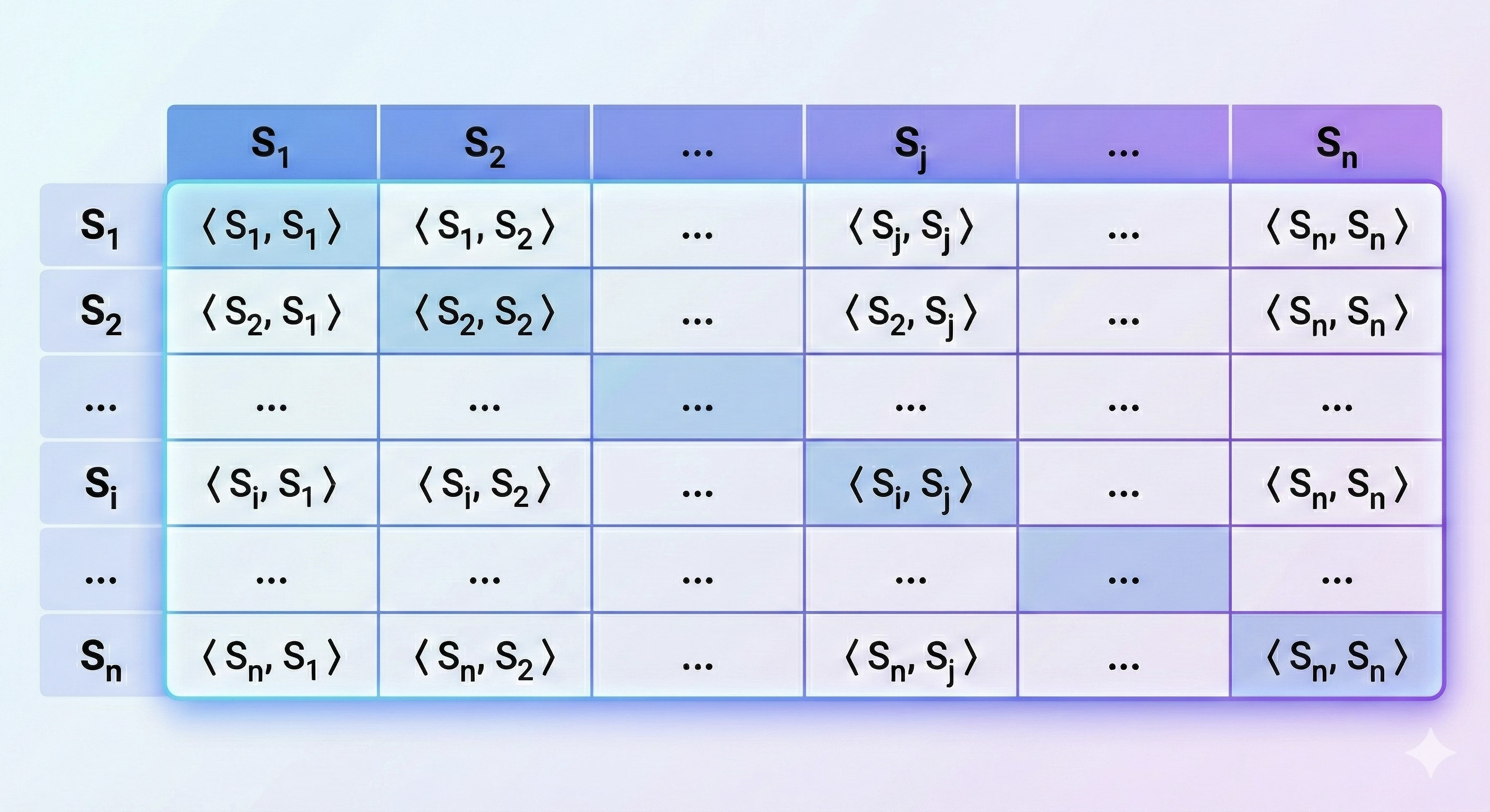
Now that we have solved the representational challenge we have all encoders (despite the differences in their output/embedding dimensionalities and misaligned vector spaces) represented by $n \times n$ matrices where $n$ is the number of sentences in $\mathcal{S}$.
It is noteworthy that selecting a representative set of sentences as $\mathcal{S}$ is an important decision we must make. For example, if $n$ is too small, then we will loose much information about the vector space (thus the encoder) represented by the PIP matrix. Mathematically, we should select a large enough set of sentences at least as the largest rank of any of encoders we would like to map. Because the rank of the vector space spanned by an encoder is equal or less than the dimensionality of the embeddings produced by that encoder, we can select $n$ to be more than the largest dimensionality of any encoder we want to put in our encoder map. However, this is only a necessary condition and not a sufficient one for PIP matrices to capture all semantics expressed by an encoder. We would need much larger set of sentences than just the maximum taken over all dimensionalities in practice. In the map of 1101 encoders we create in our paper, our largest dimensionality of any encoder is 4096. We empirically show that using 10,000 sentences is sufficient for capturing the semantics expressed by all encoders we considered. Increasing $n$ beyond 10,000 did not produced significant differences in our maps or in the downstream task performances predicted using the feature vectors created using those PIP matrices (see next section for further details about how these features are computed). However, even if the set of sentences is large but does not have sufficient diversity/coverage over linguistic phenomena unique to a language, we cannot be certain that the PIP matrix computed over those sentences will faithfully represent the semantics of the corresponding encoder. To address this issue we have to select high quality sentences (not grammatically incorrect or nonsensical ones). We sample sentences from a high quality English sentence set in our experiments. However, that would still not guarantee that we capture all possible semantic variations in English, but at least we tried not to selected a biased sample.
One can think of sentences as sensors that act on the encoder to obtain information about the semantics captured by that encoder. They do this by measuring similarity (inner-product) at various points in the (possibly infinite) language space (i.e. the space spanned by all sentences we can generate from the words in a language). That poses an interesting question about what is the possible semantic spaces that can be expressed by a given encoder? There are already prior work on compressed sensing for word embedding spaces (Arora+ 2018), which we would like to direct the interested readers. We think of PIP as a map (here we use the mathematical functional sense of map) from encoders to matrices, the million dollar question is whether PIP function is an injective map? – i.e. do we always get different PIP matrices for the different encoders? This is important given that PIP matrix will be the sole representative of an encoder going forward when we map encoders onto our encoder map – we do not want two very different encoders to be mapped close to each other in the map simply because PIP matrices were identical for those two encoders. The surjectivity of the PIP transformation is less important in our case as we can have many trivial variant of PIP matrices such as for two encoders that differ by an orthogonal projection. If we exclude those pathological cases however, we can derive a bound on the probability for PIP transformation to remain bijective (see paper for a detailed mathematical analysis). Note that the invertibility of the PIP matrix (which is square) has nothing to do with the PIP transformation being bijective or otherwise because it is not a linear transformation.
Solving the Comparison Challenge
Now that we have a representation (specifically a PIP matrix) for each encoder, we are ready to tackle the next challenge – how can we measure the distance between two encoders? This boils down to measuring some distance (alternatively similarity) metric defined over matrices. Given that all our PIP matrices representing all encoders are of the shape $n \times n$, this might appear at a first glance not a very difficult task. We indeed have many options here. Lets discuss each one of those below and see why they are not so great as they appear to be on the first glance.
- Linearising the matrices and computing $\ell_1$ or $\ell_2$ distances over the obtained vectors: We can basically “open-up” a matrix by concatenating (or horizontally stacking) each row of a PIP matrix to obtain a long vector of $n^2$ dimensions. We already have various metrics to measure distance between two vectors, which we can use for this purpose. The issue however is that we loose the periodic nature of rows – the column structure is lost in this linearised representation. This is a very heavy price to pay and a waste of effort put into creating PIP matrices in the previous step. Computing Frobenius norm is also problematic for the same reason as it simply considers corresponding elements between two matrices, ignoring the periodicity of the row/column structure. An important point worth mentioning here is that by construction, PIP matrices are symmetric. Moreover, if the embeddings were $\ell_2$ normalised, then the diagonal of all PIP matrices would simply be filled by ones, which would artificially make all PIP matrices closer to each other under such elemetwise comparisons. So this approach clearly does not cut it. One could also create vectors out of matrices by applying pooling operations such as mean pooling over rows (or columns as PIP matrices are symmetric). That would preserve periodicity but we have already created summary statistics by applying mean operation, which itself is a lossy choice.
- Centered Kernel Alignment (CKA): We can simply multiply the two PIP matrices and take the trace of the product. This can be seen as an operation that consider all elements from both matrices (map), followed up by a reducing operator (addition). However, the product (as well as the final summation) will be affected by trivial transformations such as multiplying all elements in one (or both) matrices. Clearly, the distance between two encoders should not be affected because one encoder’s embeddings are multiplied by a constant scaling factor.
- Canonical Correlation Analysis (CCA): CCA has been used in prior work for comparing the weight matrices learnt by neural nets. The original formulation uses activation scores and apply Singular Value Decomposition (SVDCCA) to make a more robust estimate, less affected by noise. These methods can potentially be applied to compare PIP matrices as well, but they are proposed and used specifically for comparing the internal representations of neural nets. In our work, we are interested in comparing encoders using the embeddings produced using those encoder rather than looking into their internal representations. This has several benefits. To begin with, not all encoders are neural network-based (e.g. one can compute sentence embeddings as a weighted pooling over static word embeddings), and activations will not be even available in the first place. Moreover, even for the encoders which are neural network-based, they might have very different architectures, complex connections, different numbers of layers, non-linearities between layers etc., which can all make things very complicated especially when comparing a map over 1000+ encoders. We would prefer a black box setup where we do not care how each encoder is designed, but how different the embeddings they produce. This can be seen as an extrinsic behavioural treatment of encoders rather than an intrinsic internal one.
OK. That depicts a gloomy picture. 😭 but do not worry… quantum information theory comes to our rescue! 🦸♂️
Before we dive into the quantum version, lets revisit the more familiar cousin in the NLP domain – relative entropy (aka. KL-divergence). If we had probability distributions instead of PIP matrices representing our encoders, then we could measure distance (technically it is divergence and not distance) using KL-divergence. Luckily for us, there is an extension of it that can be applied to density matrices given as follows:
It is worth taking a moment to look at this equation, which defines the Quantum Relative Entropy (QRE), $S(\mathbf{\rho} \Vert \mathbf{\sigma})$ between two density matrices $\mathbf{\rho}$ and $\mathbf{\sigma}$. Density matrices are obtained by simply dividing the corresponding PIP matrix by its trace, akin to normalising histograms such that they become calibrated probability distributions that adds up to one. $$S(\mathbf{\rho} \Vert \mathbf{\sigma}) = \mathrm{Tr}(\mathbf{\rho} \ln \mathbf{\rho}) - \mathrm{Tr}(\mathbf{\rho} \ln \mathbf{\sigma})$$ The first term is very similar to the self-entropy term in KL-divergence (and indeed known as the Shanon entropy), whereas the second term corresponds to the cross-entropy between the two density matrices. One important caveat here is that the logarithms (ln) are taken not in an elementwise manner but over the eigenvalues of the density matrices.
In theory, we have a divergence measure between two PIP matrices (by extension the encoders corresponding to those PIP matrices), so we have solved the comparison challenge! 🎉 But I am afraid, the reality is not as forgiving as that. As we have seen several times already in this article, different encoders live in different eigenspaces that are all subsets of the $n$ dimensional vector space. When the eigenspaces of the two density matrices do not align (does not contain the same set of eigenvectors) QRE goes to infinity. Lets first see why this happens in the three dimensional example below.
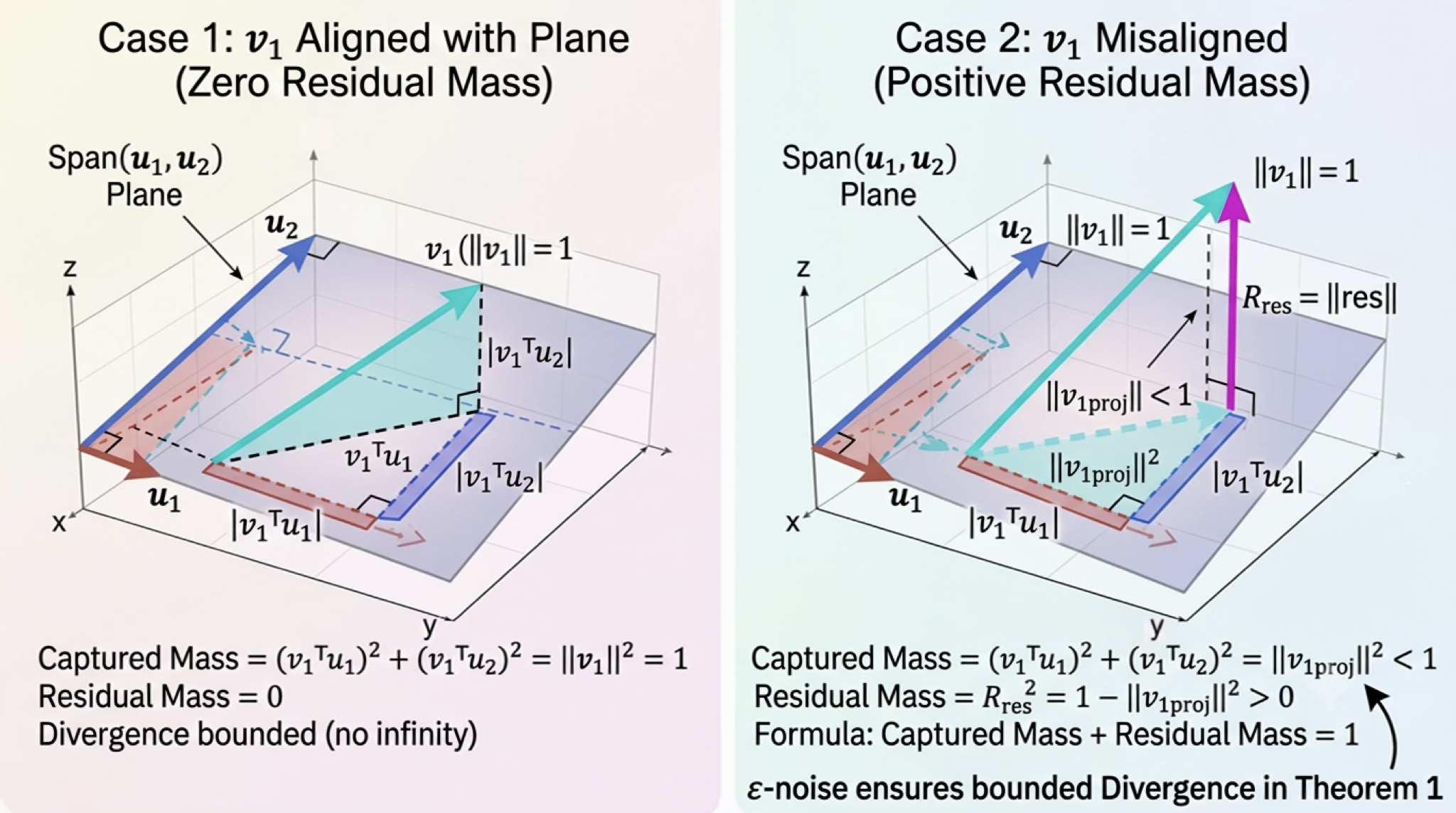
Let us consider the situation where one encoder has two eigenvectors $u_1$ and $u_2$, whereas the other has one eigenvector $v_1$. In case 1 (shown on the left), we have $v_1$ on the plane spanned by $u_1$ and $u_2$ (i.e. $v_1$ can be expressed as a linear combination of $u_1$ and $u_2$). In this case, according to Pythagorus theorem, we can perfectly reconstruct $v_1$ (which has length of 1 by construction) using its projections onto $u_1$ and $u_2$. However, when $v_1$ does not lie on this plane (as shown in case 2 on the right), the squared sum of projections will be less than 1, which implies some amount of probability mass will be “lost”. Unless we put this missing (residual) mass back into the QRE calculation it will not be properly defined.
This is quite analogous to the situation in KL divergence where it is undefined when the probability distributions compared have different domains. When one distribution is not defined at a point where the other is, then cross-entropy term will be undefined (or if we consider log to diverge to negative infinity when the input goes to zero). In the case of KL divergence, the standard trick is to “smoothen” the probability distributions such that they remain non-zero in the union of the domains of each distribution. For example, Jensen-Shanon divergence is computed against $(p+q)/2$ for two probability distributions $p$ and $q$, which would guarantee that the base distribution remains defined on all inputs where $p$ and $q$ are defined. A similar extension can be applied for QRE as well – we can “smoothen” the eigenvalues by adding a small perturbation noise $\epsilon > 0$. However, recall that we cannot just perturb eigenvalues by ignoring their corresponding eigenvectors. In this particular case, we are perturbing the null space (i.e. eigenvectors that correspond to zero eigenvalues). Therefore, this requires reinstating those missing null vectors back into the eigenspaces of the density matrices. For a more mathematical treatment of this issue alongside with the solution we propose please refer to the ACL paper.
Although QRE provides a pairwise measure of divergence between two encoders, we must select some base point for creating our map. In other words, the distances all must be computed with respect to the same starting point to create a map. We could simply select one of the encoders as this base point (aka base encoder). However, doing so could bias all our measurements to the chosen base encoder. To avoid such selection biases for the base encoder, we propose to use an uninformative prior where we use the basis vectors (i.e. 1-hot embeddings which spans the $n$ dimensional vector space), which we call the unit base encoder. Under this base encoder we show that each dimension corresponds to a feature that contributes independently to the total QRE value. This is nice because it provides us with a coordinate space (albeit $n$ dimensional) for representing all encoders. This feature vector representation can be used to represent any encoder and can be used to predict downstream task performance of that encoder. Moreover, the $\ell_1$ distance computed between two encoders in this feature space (approximately) calculates the QRE of one encoder given the other. We like to have 2D maps for convenience. Therefore, we apply t-SNE to project encoders from $n$ to $2$ dimensions, producing the maps we discuss in the next section.
What do the maps tell us?
Lets take a closer look at some of the maps produced by the above-described method.
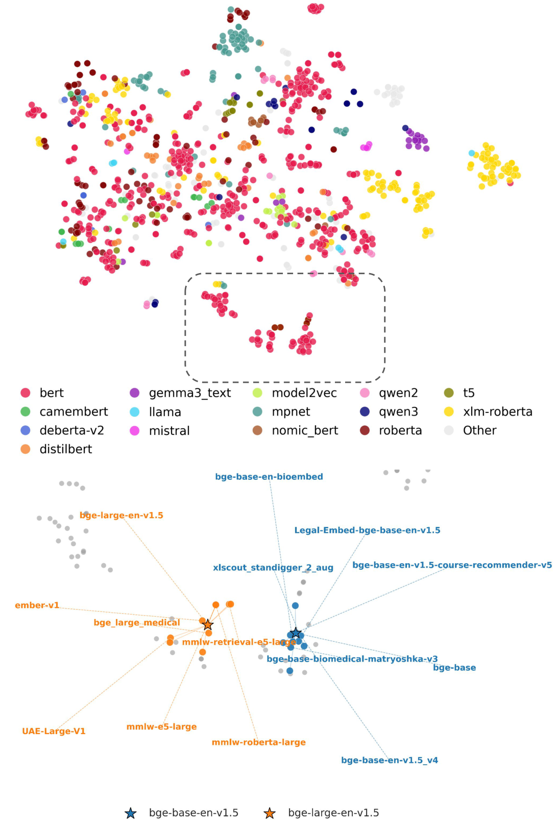
Top: Map for 1101 sentence encoders, visualised by t-SNE and coloured by the encoder type. Bottom: A 30% zoomed-in view of the dotted area showing the top-7 nearest neighbours for bge-base and bge-large. Nearest neighbours belong to the same primary architecture and are closely located.
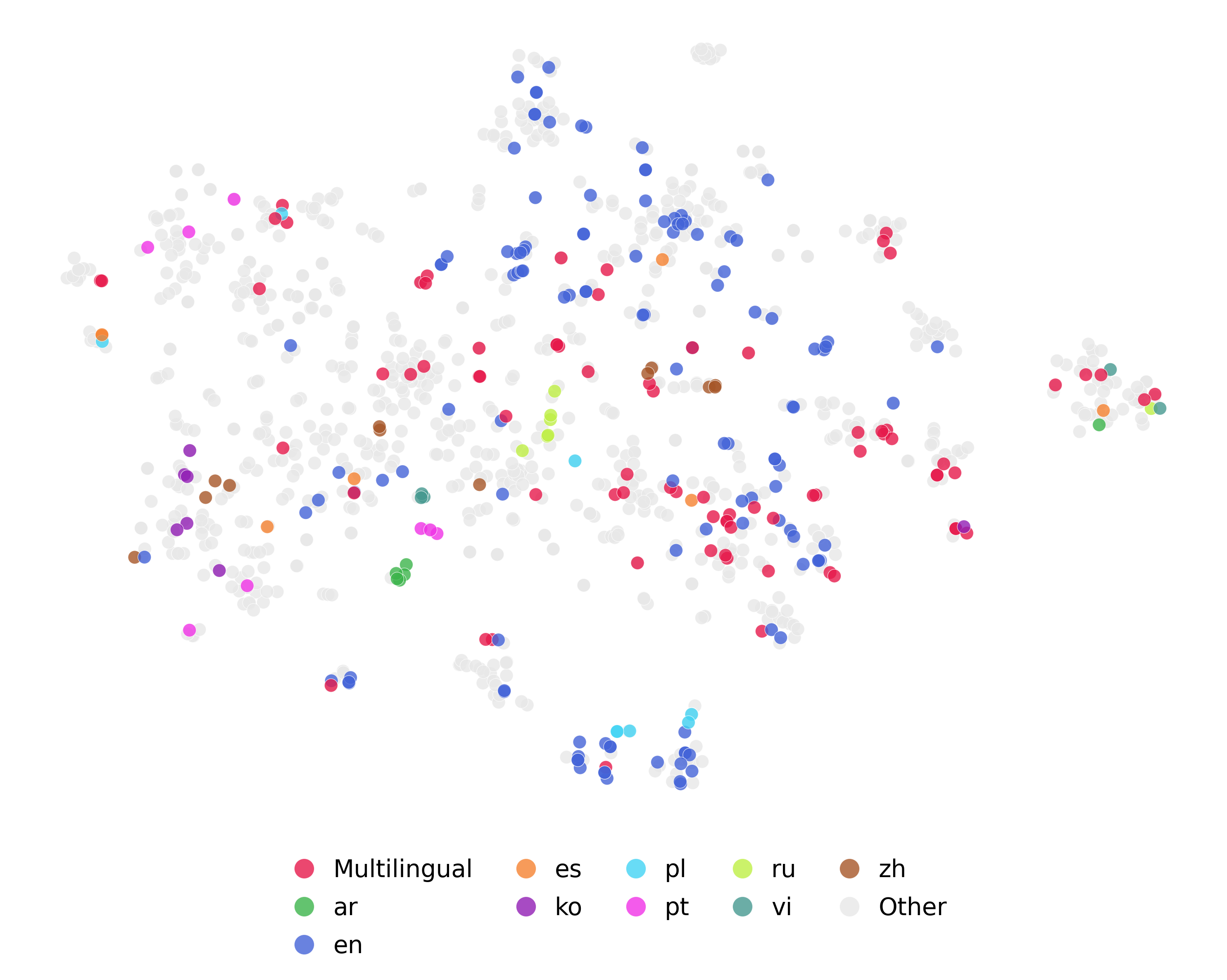
Encoders coloured by the pretraining language. Encoders trained only on English (en) are mostly located at the central portion of the map spanning from top to bottom, whereas encoders trained on multilingual datasets are located at the centre and right side of the map. Note that most of the mul-tilingual datasets contain English. Monolingual encoders (except English) such as for Arabic (ar) and Korean (ko) languages can be found in concentrated clusters.
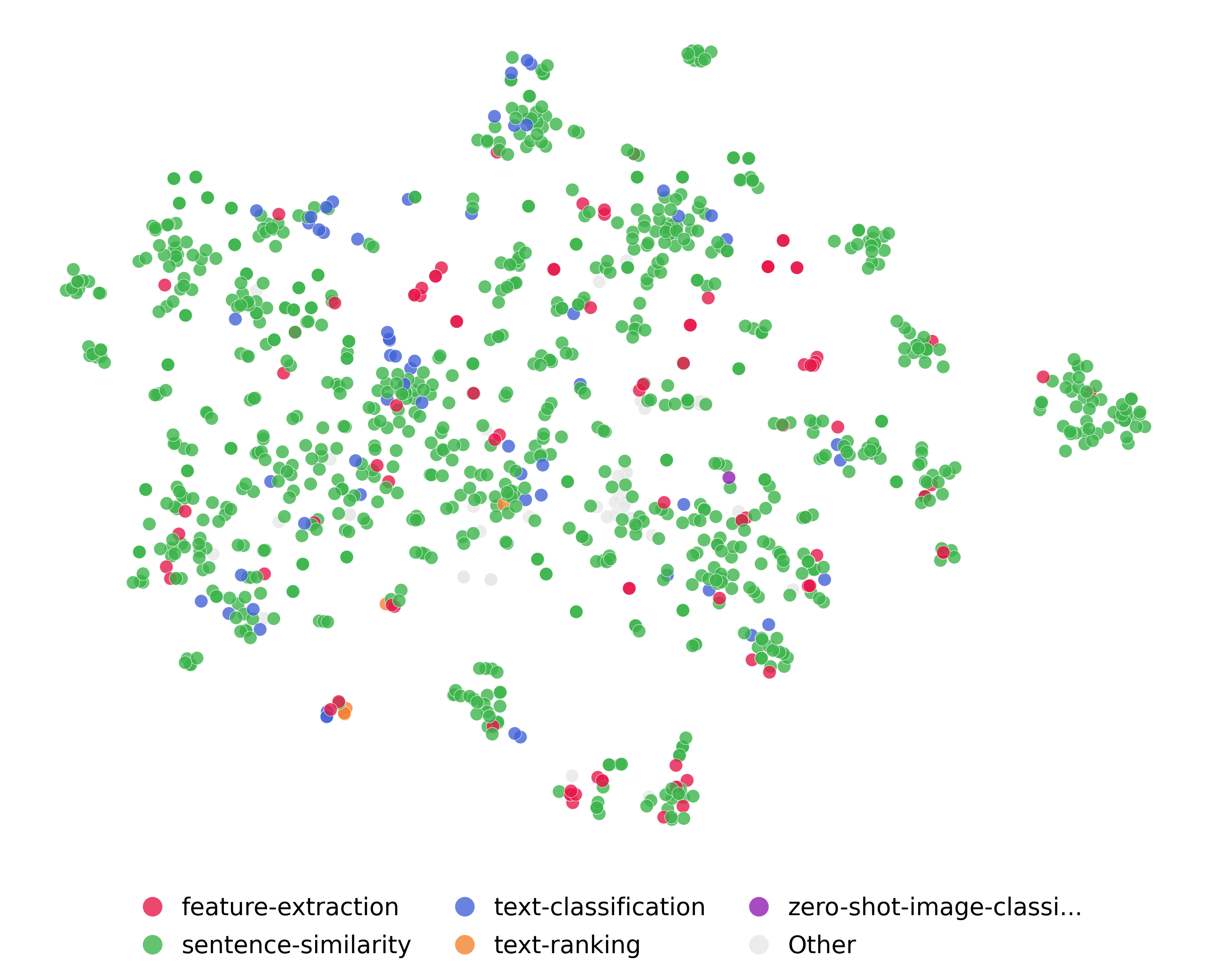
Fine-tuning tasks used for training the sentence encoders. We see that all encoders are mostly fine-tuned on the sentence similarity tasks, a standard fine-tuning task for sentence encoders showing its prevalence on the map. Feature extraction and text classification are also commonly used tasks for fine-tuning encoders. Although they are not as prevalent as sentence similarity task, they are also spread throughout the map.

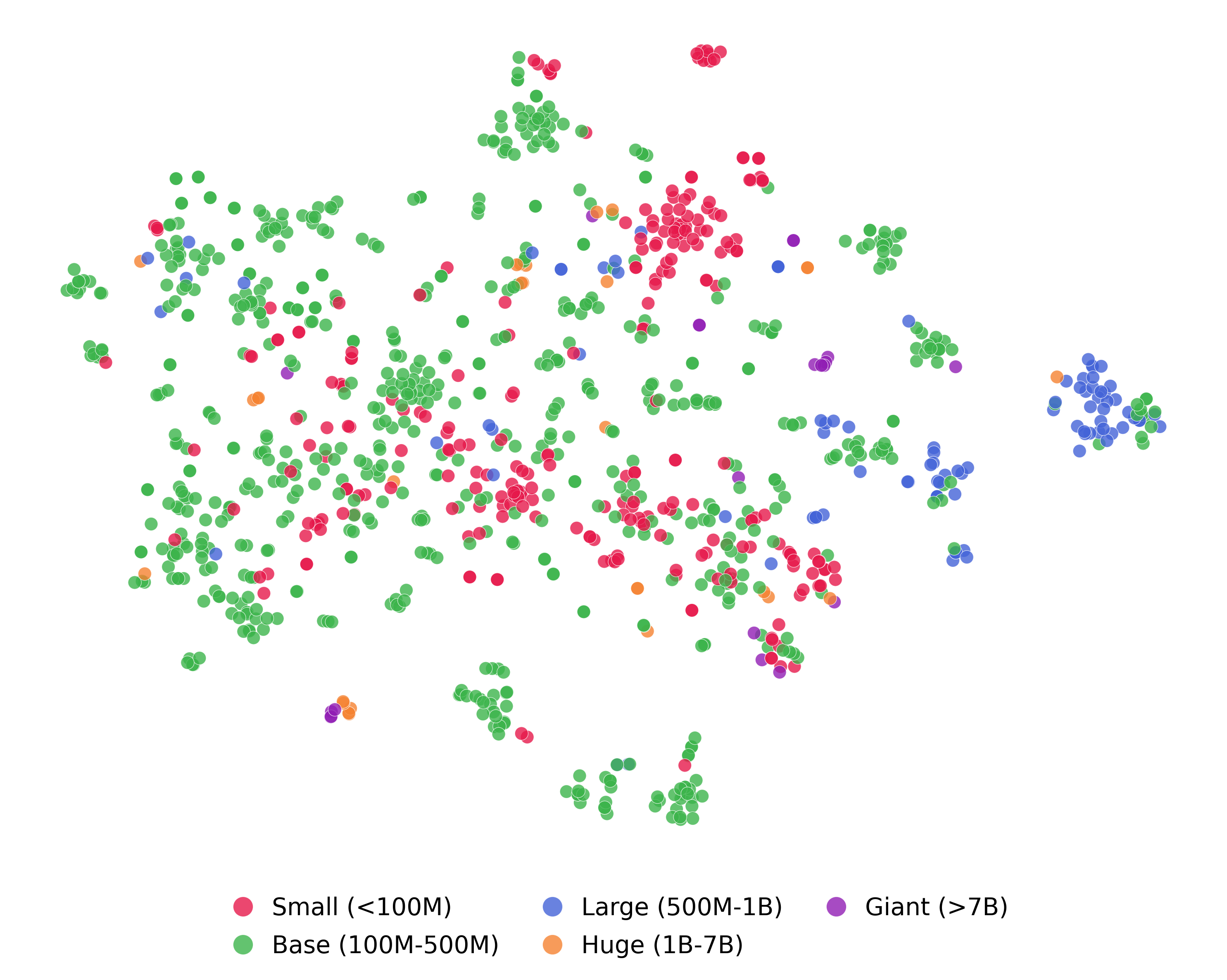
Encoders coloured by the number of parameters. We see that encoders with smaller parameter sizes (<100M) tend to cluster at the middle and top, whereas encoders with larger parameter sizes (500M-1B) cluster on the far right side. Encoders with parameter sizes (>1B) tend to be scattered across the map, instead of forming tight clusters. This might be because smaller models are often distilled or fine-tuned from the larger foundation models, making them similar to each other on the map. For example, a closer look at the map reveals that the Qwen series encoders with different parameter sizes are closer to each other on the map (e.g. 8B, 4B and 0.6B).